Civic Data Atlas

• Home
• More

Methodology

Data Sources

American Community Survey

Most statistics come from the American Community Survey (ACS). The ACS is a large, high-quality nationwide survey conducted by the U.S. Census Bureau. In 2024, the ACS response rate exceeded 80%, and the total sample included nearly 2 million households.

ACS 5-Year Estimates

We use the ACS’s 2024 5-Year Estimates, which draw from surveys conducted from 2020 through 2024. The 2024 5-Year Estimates are the latest 5-year data available; the 2025 5-Year Estimates should be available in early 2027.

Ideally, we would use more recent data rather than aggregating five years of survey responses, some of which are several years old by the time the estimates are released. However, only 5-year estimates have a large enough sample to compute statistics at the local district or neighborhood level.¹ On the city homepages, the four summary cards use ACS 1-year estimates instead, since citywide sample sizes are large enough to support the more current release.

Census LEHD Origin-Destination Employment Statistics

Some job and commuting-related statistics come from the U.S. Census Bureau’s Longitudinal Employer-Household Dynamics (LEHD) Origin-Destination Employment Statistics (LODES). LODES is an administrative data product, not a survey. It is built primarily from state Unemployment Insurance wage records, supplemented by federal employment records.

LODES counts a job when the worker has positive earnings in both the reference quarter and the preceding quarter. The 2023 data used here refers to the second quarter of 2023. LODES is typically updated annually, with a two- to three-year lag.

Although LODES is based on administrative records rather than a survey, it still has sources of imprecision. Its Unemployment Insurance records cover most wage-and-salary jobs reported through state Unemployment Insurance systems, but exclude self-employed workers and other employment not covered by Unemployment Insurance, including military, railroad, certain agricultural, nonprofit, and family employment. Some federal jobs are included, but federal coverage is incomplete.

Locations of job sites are reported by employers, but some employers do not report multiple worksites separately. In those cases, the Census may assign all of an employer’s workers in a state to the employer’s main reported address. Workers’ home locations come from a variety of federal administrative sources, including tax returns, U.S. Postal Service change-of-address records, and benefits-enrollment records. Although LODES attempts to match a worker’s residence to the period of the linked job, a recently moved worker may be assigned an address that does not reflect their residence at the job’s reference date. Finally, LODES uses noise infusion and synthetic-data techniques to protect the confidentiality of the underlying records, so published statistics may differ from the confidential underlying counts, particularly at fine geographic levels. More details on the methodology are available here.

CDC PLACES

Statistics on health conditions come from the U.S. Centers for Disease Control and Prevention’s PLACES data. The CDC PLACES data comes from a combination of the Behavioral Risk Factor Surveillance System Survey (BRFSS) and the American Community Survey (ACS). The BRFSS surveys over 400,000 people every year on a range of health topics. While it is a large survey, it is not large enough to estimate health statistics at a hyperlocal level. To produce reliable local estimates, the CDC combines BRFSS and ACS data using a technique called multilevel regression and poststratification modeling.

For each census tract, ACS data describes the demographic composition of the local population, including residents’ age, sex, race and ethnicity, and educational attainment. BRFSS data is then used to estimate how the prevalence of different health conditions varies across those demographic groups. Multilevel regression and poststratification combines these two sources by applying BRFSS-based health estimates to the demographic profile of each tract. Essentially, the prevalence of various health conditions in a tract is predicted based on the tract’s demographic characteristics from the ACS.

The CDC PLACES data was last published in 2025 and is based mostly on data from the 2023 BRFSS survey and the 2019–2023 ACS. Five measures are based on 2022 BRFSS survey data: 1) Colorectal cancer screening, 2) Mammography, 3) Short sleep duration, 4) Dental visit, and 5) All teeth lost. CDC PLACES data is updated annually.

Unlike the survey-based estimates elsewhere on this site, CDC PLACES values are modeled estimates, and the CDC does not publish a margin of error for them. We therefore do not show a margin of error for any CDC PLACES measure. One measure, the share of adults who have lost all their teeth, is only asked of adults 65 and over; we express it as a share of all adults 18 and over so it is comparable to the other measures, which are reported for all adults 18 and over.

HUD Picture of Subsidized Households

Housing assistance data on the neighborhood and district pages comes from the U.S. Department of Housing and Urban Development’s (HUD) administrative dataset, the Picture of Subsidized Households. The Picture of Subsidized Households is not a sample-based survey. Instead, it aggregates administrative data from local housing authorities that administer HUD-funded housing assistance programs. All people receiving HUD-funded federal housing assistance are included in the data.² HUD’s Picture of Subsidized Households uses 2025 data and is updated every year.

Census Local Air Conditioning Estimates

Estimates of air conditioning access come from the U.S. Census Bureau’s Local Air Conditioning Estimates (LACE). These estimates come from combining local data from the American Community Survey with national data on air conditioning access from the American Housing Survey (AHS), also administered by the Census Bureau.

The American Housing Survey does not have a large enough sample to provide estimates of air conditioning access at a hyperlocal level. To produce reliable local estimates, the Census combines AHS and ACS data similarly to how the CDC combines BRFSS and ACS data. In this context, the Census uses individual survey responses from the ACS rather than ACS data aggregated to the tract level. Thus, rather than predicting tract-level outcomes from an area’s demographics, the model predicts AC access for each household based on that household’s characteristics, then aggregates the predicted AC access to the tract level using an approach called cross-survey modeling.

The Census Bureau’s local air conditioning estimates were released in 2026 but refer to data collected in 2023. Since these estimates are new, it is not yet clear how often the Census will update them.

Census Community Resilience Estimates for Heat

Estimates of community resilience to heat come from the U.S. Census Bureau’s Community Resilience Estimates (CRE) for Heat dataset. The data is designed to show a community’s vulnerability to extreme heat by defining and tabulating the average number of social vulnerability measures present in the community. The vulnerability measures come directly from the American Community Survey. Unlike the Local Air Conditioning Estimates and CDC PLACES data, the CRE for Heat data does not rely on cross-survey modeling. The specific social vulnerability measure definitions are described in detail on our social vulnerability definitions page.

The Census Bureau’s Community Resilience Estimates for Heat data was published in 2024 and refers to data collected in 2022. Historically, the data has been updated every three years.

Tree Canopy and Land Cover

Tree canopy and land cover measures come from the National Baseline Assessment of Urban and Community Forests, a 2026 assessment developed by the USDA Forest Service Urban and Community Forestry Program in partnership with the Arbor Day Foundation and PlanIT Geo. The assessment uses high-resolution aerial imagery to classify land cover across U.S. communities. Land cover data is based on USDA National Agriculture Imagery Program imagery collected from 2021 to 2023 during leaf-on conditions. Using machine learning, the source data classifies each census block group into six land cover classes: tree canopy, shrub, herbaceous vegetation, impervious surface, soil, and water. Civic Data Atlas combines shrub, herbaceous vegetation, soil, and water into a single category called “natural open surfaces.” Because this is a new data source, its update schedule is unclear.

Opportunity Atlas

Data on the adult outcomes of children who grew up in a given district or neighborhood come from The Opportunity Atlas, a dataset of economic mobility outcomes across the United States. The Atlas is a collaboration between researchers at the U.S. Census Bureau and Opportunity Insights, a group of academics at Harvard University. The underlying data comes from de-identified federal income-tax returns linked to the decennial Census, covering nearly the entire U.S. population born between 1978 and 1983. For each district or neighborhood, the data follow children who grew up in that location. Adult outcomes are measured primarily using tax returns from 2014 and 2015; incarceration is measured using data from April 1, 2010. As adults, the people followed from childhood could live anywhere in the United States—the data follows all children of a given location, not those that remained in the same place as adults.

Neighborhood Boundaries

Chicago’s 77 neighborhoods come from the city’s official Community Areas boundaries. New York City’s 197 neighborhoods are the Department of City Planning’s Neighborhood Tabulation Areas (NTAs). Los Angeles’s 110 neighborhoods come from the City of Los Angeles’s GeoHub open data portal, and use neighborhood boundaries originally created by the Los Angeles Times.

Geographic Aggregation

Plain-English Summary

Local district and neighborhood statistics are not precomputed by the Census Bureau or other statistical agencies. It is also not possible to simply aggregate survey responses from people within a given district or neighborhood from Census data: the Census Bureau does not reveal respondents’ precise geographic locations. To compute these statistics, we aggregate data from smaller geographic areas that fall within or overlap a given neighborhood or district, using the most granular geographic information the statistical agency releases. Some of these areas do not perfectly align with district boundaries: part of the area may be inside the district, while another part is outside of it. When this occurs, we weight the data by the fraction of the area’s population that falls within the district boundaries. While this geographic mismatch is unavoidable, validation tests suggest that it has a very small impact on the accuracy of the resulting statistics. For the subset of metrics where we can test the effect of imperfect boundary overlap, average errors are less than half of one percentage point.

Aggregating Across Census Geographies

Local district and neighborhood statistics are not precomputed by the Census Bureau. To calculate them, we take a weighted average of smaller geographic units, called census tracts, that fall within or overlap a district or neighborhood. For readability, the examples below refer to census tracts and districts. However, the same procedure applies to neighborhoods, and the actual calculations use the smallest available geography for each measure: block groups when block-group data is available, and tracts otherwise.

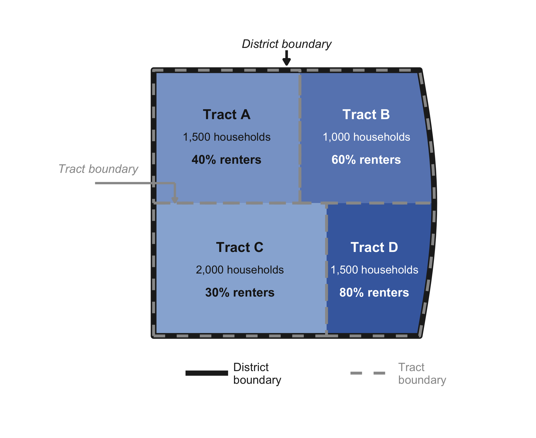
As a simple example, consider calculating the percentage of renter-occupied households in a district with four census tracts, each of which is fully within the district boundary:

To find the district-level renter percentage, we take the weighted average of the tracts’ renter shares, weighting each tract by its total number of households:

District renter %  =  (pop_A × renter%_A) + (pop_B × renter%_B) + (pop_C × renter%_C) + (pop_D × renter%_D) pop_A + pop_B + pop_C + pop_D

 =  (1,500 × 40%) + (1,000 × 60%) + (2,000 × 30%) + (1,500 × 80%) 1,500 + 1,000 + 2,000 + 1,500  =  50.0%

Dealing with Imperfect Overlap Between Tracts and Districts

In practice, census tract boundaries do not always align with district boundaries: some tracts include residents from multiple districts. For split tracts, we use the data for the full tract, including residents living both inside and outside the district boundary. We account for the fact that some residents live outside the district by weighting the tract by the fraction of its population falling within the district boundaries, rather than using the tract’s total population.

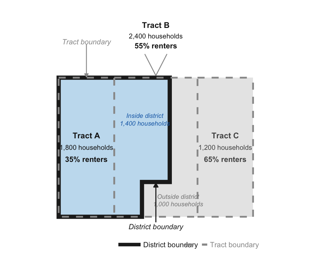
For example, the figure above shows a district boundary that fully encompasses Tract A but only partially overlaps Tract B. When calculating the district’s renter share, we know that 35% of households in Tract A are renter-occupied and that 55% of households in Tract B are renter-occupied, but we do not know the renter share for the portion of Tract B inside the district. However, we do know how much of Tract B’s population is inside versus outside the district. We account for this by weighting Tract B’s renter share by the population of Tract B inside the district, 1,400 households, rather than by its full population, 2,400 households.

District renter %  =  (pop_A × renter%_A) + (pop_{B, in district} × renter%_B) pop_A + pop_{B, in district}

 =  (1,800 × 35%) + (1,400 × 55%) 1,800 + 1,400  =  43.8%

We calculate the share of each split census tract’s population within the district using block-level data from the 2020 decennial Census. Census blocks are very small and almost always fall entirely within a single district.³ The figure below shows how block-level population data can be used to weight split tracts, using the example from Tract B above.

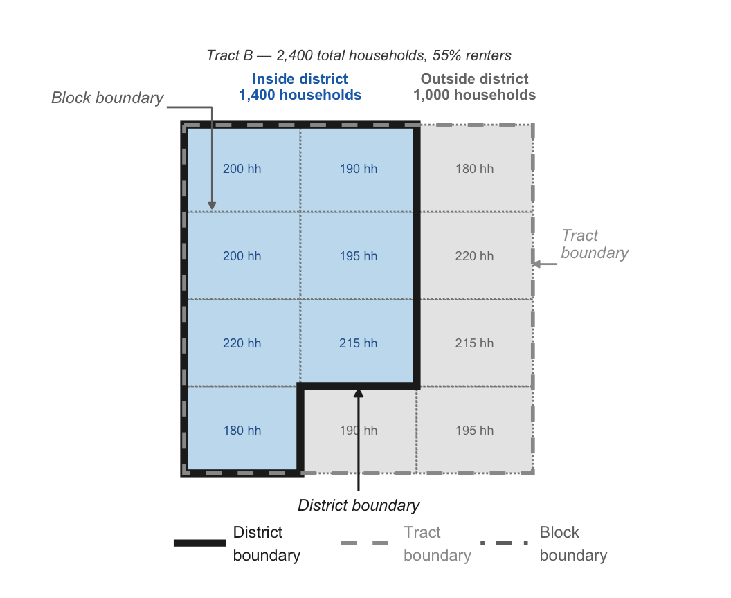
Importantly, only a handful of basic variables, such as population and housing-unit counts, are available at the block level. While we have total population data at the block level from the 2020 decennial Census, renter share and most other ACS variables are available only at higher levels of aggregation. As a result, we must use the tract-wide renter percentage rather than the renter percentage for the portion of the tract within the district boundary.

Handling Change Over Time Calculations

Changes in Census Geographies

To track a district’s or neighborhood’s change over time, we want to compute statistics from the same geographic area at different time points. Already we have to deal with the fact that census geographies don’t perfectly overlap neighborhoods and districts—a complication covered in the last section. A further complication is that the Census Bureau redraws some census tracts and block groups after each decennial census. This means some change-over-time comparisons may be based on slightly different geographic areas over time. In other words, some degree of change over time may not be a true change in demographics for a given district or neighborhood, but simply a change in the underlying census tract geography that best approximates a district or neighborhood boundary. For historical comparisons, change over time statistics will extra geographic aggregation error caused by a combination of census - geographic area mismatch and census boundary changes over time.

Fixed Geographies

All change-over-time statistics hold geography fixed—we match the current-day district or neighborhood boundaries to historical data to estimate the change over time for the same geographic area. In other words, we ignore the fact that district boundaries were different in the past—we try to match historical data to present-day boundaries so as not to conflate changes over time with changes in geographic boundaries.

When we compute change over time for districts or neighborhoods that have had census tracts or block groups redrawn, we try to match the best-fit 2020 Census geographies, not the actual district boundaries. While in some cases, historical block groups and tracts may be better able to match district boundaries than current ones, we want to try to isolate change over time in a constant geography, using the best representation of the district from 2020 Census data that we can get.

Sources of Error and Imprecision

Sampling Error

The ACS surveys a sample of households rather than every household in the country. Because the ACS captures only a slice of the population, any statistic it produces is an estimate — and like all estimates, it comes with some uncertainty. If the ACS were conducted again with a new sample of households, it would yield slightly different results. This sample-to-sample variation is called sampling error, and it exists for all surveys.

A survey’s margin of error quantifies the uncertainty from sampling error. It defines a range around the published estimate within which the true population value is likely to fall. For example, if a district has an estimated renter-occupied household share of 42%, with a margin of error of ±4 percentage points, the true value is likely between 38% and 46%.⁴ ACS margins of error are reported at the 90% confidence level, meaning that if the survey were repeated many times, the true value would fall within that range about 90% of the time. Each district page has a button that allows users to toggle margins of error on or off for each estimate. Technical details on how we compute district-level margins of error from ACS tract and block-group data are described on this page.

Geographic Aggregation Error

When a tract overlaps a district boundary, our calculations necessarily incorporate some data from people living outside the district. This introduces geographic aggregation error — a source of imprecision distinct from sampling error. Unlike sampling error, geographic aggregation error is not directly quantifiable from the published ACS data.⁵ The degree to which a district is mismeasured by incorporating non-district residents depends on how different those non-district residents are from district residents, which is unknown.⁶

While we cannot directly test geographic aggregation error in the ACS estimates, we can test it using block-level decennial Census data. Since census blocks are very small, we can use them to produce district-level estimates without geographic aggregation error. Using the same data, we can compute district-level estimates with geographic aggregation error by applying the same methodology we use on the ACS data.⁷ Comparing district estimates from block-level data aligned directly to district boundaries with estimates produced using our tract- and block-group aggregation method allows us to quantify how much imperfect geographic overlap between Census and district boundaries can skew estimates.

For each district, we show the geographic mismatch between Census boundaries and district boundaries, as well as validation tests using decennial Census data with and without geographic aggregation error. The table below summarizes the mismatch error for each city a geography type. Overall, average errors are very small—always less than half a percent, and typically much smaller.

Geography	Hybrid	Tract-only
Chicago wards	0.22 p.p.	0.34 p.p.
New York City council districts	0.05 p.p.	0.13 p.p.
Los Angeles council districts	0.04 p.p.	0.06 p.p.
Chicago community areas	0.01 p.p.	0.02 p.p.
New York City neighborhoods	<0.001 p.p.	<0.001 p.p.
Los Angeles neighborhoods	0.19 p.p.	0.40 p.p.

Importantly, decennial Census data is available for only a small number of measures, including race, age, owner- versus renter-occupied households, and household types.⁸ However, geographic aggregation error in measures included in the decennial Census may differ from the error in other ACS measures. For instance, the portion of a split tract inside the district may have a similar renter share to the portion outside the district, a measure available in both ACS and decennial Census data, while rent prices may differ substantially across the same boundary, a measure available only in the ACS.

Change Over Time Error

As some census tracts and block groups are redrawn over time, we are forced to use data that represents a slightly different geography than in past years then present years for some geograpies. This can mean some computed changes over time could be specious, caused by geographic boundary changes rather than true changes in the underlying population.

We can test the degree to which census boundary changes over time distrort change over time statititcs using a validation exercise similar to what we do for present day geographic aggregation error. For each district, we use decennial Census block data to compute demographics using 2020 Census geographies as well as our best-matching 2010 Census geographies. At the block level, we can compute demographic statistics for both sets of geographies with near-perfect accuracy because census blocks are very small. Holding the underlying data fixed, we can then see how demographics differ when approximating district boundaries using 2020 census geographies vs 2010 census geographies. Across cities, differences are very small, as shown in the table below. For almost all cities, change over time errors are smaller than present day geogrpahic aggregation error, and always less than .1 percentage point.

Geography	Hybrid	Tract-only
Chicago wards	0.010 p.p.	0.022 p.p.
New York City council districts	0.036 p.p.	0.041 p.p.
Los Angeles council districts	0.015 p.p.	0.020 p.p.
Chicago community areas	0.002 p.p.	0.002 p.p.
New York City neighborhoods	0.011 p.p.	0.041 p.p.
Los Angeles neighborhoods	0.059 p.p.	0.096 p.p.

Self-Report Errors

ACS data comes from self-reported responses, which are subject to error. The degree to which this matters varies by question. For instance, most people can accurately report their age, but when asked the year their building was constructed, respondents may give their best estimate rather than a precise answer. More broadly, the accuracy of survey data depends on the reliability of self-reported responses. For questions like building age, answers should be understood as rough approximations rather than precise measurements. We try to account for this in how we present the data. For instance, our housing age variable uses wide bins that convey the rough age distribution of the housing stock, such as relatively new, middle-aged, and older buildings, rather than precise construction dates.

Footnotes

1. The Census does not release precise geographic information from the American Community Survey to protect the privacy of respondents. To calculate neighborhood or district-level statistics, we have to aggregate data across the geographies that the Census Bureau does release. The smallest published geographic units typically include only 1,200 to 8,000 people, and there are not enough survey respondents within those units in a single year. The 5-year estimates combine five years of survey responses to provide more stable and reliable estimates for smaller geographies.

2. One major affordable housing program not included in the data is the Low-Income Housing Tax Credit (LIHTC), which is separate from HUD’s main rental assistance programs. One complication of LIHTC properties is that tenants often receive housing vouchers in addition to living in a subsidized LIHTC building. HUD’s data is not detailed enough to identify these households that are receiving more than one type of subsidy.

3. In the rare cases where a block straddles a district boundary, we weight the block’s population by the share of the block’s area falling within the district.

4. Not all values within this range are equally plausible. The published estimate is the single most likely value; plausibility decreases gradually toward the edges of the range, following a bell-curve distribution.

5. Arguably, sampling error also has some unquantifiable bias. Traditional margins of error are calculated based on an assumption of a random sample. In practice, not everyone who receives the ACS answers the survey, and people who respond may differ from people who do not respond. This breaks the logic of random sampling that margins of error are based on and makes the degree of total sampling error also fundamentally unknowable. However, the ACS is a very high-quality survey, with high response rates and methods designed to reduce sampling bias.

6. Population shifts within split tracts since the 2020 Census (which is the data source we use to weight split tracts by the fraction of the population inside the district) may also be a source of error.

7. Specifically, we aggregate data from census blocks up to the tract and block-group levels, then use those data the same way we use ACS data: weighting units that split district boundaries by their block-level population.

8. The ACS is far more comprehensive and surveys people more frequently than once every 10 years, which is why we use it despite the presence of geographic aggregation error.